Basic Packages - Python and Jupyter Notebook
Econ 570 Big Data Econometrics - 2nd TA session
Jupyter Notebook Basic
The Jupyter Notebook has two modes:
-
command mode: blue cell border
-
edit mode: green cell border
While in command mode (press Esc to activate)
- Enter: take you into edit mode
While in edit mode (press Enter to activate)
- Esc: take you into command mode
Shortcuts in both modes:
-
Shift + Enter: run the current cell, select below
-
Ctrl + Enter: run selected cells
-
Alt + Enter: run the current cell, insert below
-
Ctrl + S: save and checkpoint
While in command mode:
-
A to insert a new cell above the current cell, B to insert a new cell below.
-
M to change the current cell to Markdown, Y to change it back to code
-
D + D (press the key twice) to delete the current cell
** you can check more shortcuts in [ Help -> Keyboard Shortcuts ]
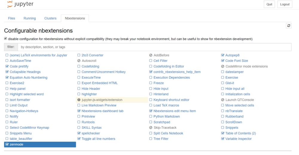
Jupyter Notebook Extensions
Jupyter Notebook extensions are simple add-ons that extend the basic functionality of the notebook environment.
How to install (Run the following in a command prompt)
pip install jupyter_contrib_nbextensions && jupyter contrib nbextension install
Based on: https://www.geeksforgeeks.org/what-is-the-difference-between-pythons-module-package-and-library/
What is the difference between Python’s Module, Package and Library?
Module: The module is a simple Python file that contains collections of functions and global variables and with having a .py extension file. It is an executable file and to organize all the modules we have the concept called Package in Python.
Example: Save the code in file called demo_module.py
    def myModule(name):
        print("This is My Module : "+ name)
Import module named demo_module and call myModule function inside it.
    import demo_module
    demo_module.myModule("Math")
Output:
This is My Module : Math
Package: The package is a simple directory having collections of modules. This directory contains Python modules and also having init.py file by which the interpreter interprets it as a Package. The package is simply a namespace. The package also contains sub-packages inside it.
Example:
Student(Package)
| __init__.py (Constructor)
| details.py (Module)
| marks.py (Module)
| collegeDetails.py (Module)
Library: The library is having a collection of related functionality of codes that allows you to perform many tasks without writing your code. It is a reusable chunk of code that we can use by importing it in our program, we can just use it by importing that library and calling the method of that library with period(.).
Example: Importing pandas library and call read_csv method using alias of pandas i.e. pd.
    import pandas as pd

    df = pd.read_csv("file_name.csv")
References
Basic packages
NumPy - http://www.numpy.org/
pandas - https://pandas.pydata.org/
statsmodels - https://www.statsmodels.org/stable/index.html#
matplotlib - https://matplotlib.org/
Websites
PyEcon - https://pyecon.org/
Learn Python - https://www.learnpython.org/
NumPy
NumPy - http://www.numpy.org/
The Numerical Python package NumPy provides efficient tools for scientific computing and data analysis:
- np.array(): Multidimensional array capable of doing fast and efficient computations,
- Built-in mathematical functions on arrays without writing loops,
- Built-in linear algebra functions.
# Create 2 new lists height and weight
height = [1.87,  1.87, 1.82, 1.91, 1.90, 1.85]
weight = [81.65, 97.52, 95.25, 92.98, 86.18, 88.45]

# Import the numpy package as np
import numpy as np

# Create 2 numpy arrays from height and weight
np_height = np.array(height)
np_weight = np.array(weight)
# Element-wise calculations
# Calculate bmi
bmi = np_weight / np_height ** 2

# Print the result
print(bmi)
[23.34925219 27.88755755 28.75558507 25.48723993 23.87257618 25.84368152]
# Subsetting
# For a boolean response
bmi > 25
array([False, True, True, True, False, True])
# Print only those observations above 23
bmi[bmi > 25]
array([27.88755755, 28.75558507, 25.48723993, 25.84368152])
# Conditional logic
# np.where(condition, a, b): If condition is True, returns value a, otherwise returns b.

a = np.array([4, 7, 5, -7, 9, 0])
b = np.array([-1, 9, 8, 3, 3, 3])
cond = np.array([True, True, False, True, False, False])
res = np.where(cond, a, b)
res
## array([ 4, 7, 8, -7, 3, 3])
array([ 4, 7, 8, -7, 3, 3])
res = np.where(a <= b, b, a)
res
## array([4, 9, 8, 3, 9, 3])
array([4, 9, 8, 3, 9, 3])
Linear algebra (numpy.linalg)
https://numpy.org/doc/stable/reference/routines.linalg.html
# Linear algebra
import numpy.linalg as nplin
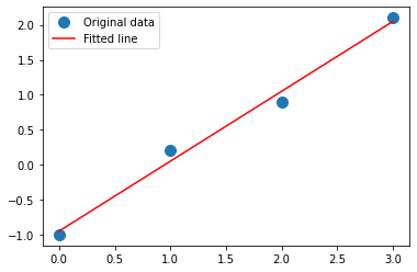
# Return the least-squares solution to a linear matrix equation.
# y = bx + e
x = np.array([0, 1, 2, 3])
y = np.array([-1, 0.2, 0.9, 2.1])

print(x)
print(np.random.rand(1,4))

# A includes constant term
A = np.vstack([x, np.ones(len(x))]).T
A,y
[0 1 2 3]
[[0.45889207 0.93171399 0.69273904 0.44251122]]


(array([[0., 1.],
        [1., 1.],
        [2., 1.],
        [3., 1.]]),
 array([-1. ,  0.2,  0.9,  2.1]))
b, e = np.linalg.lstsq(A, y, rcond=None)[0]
b, e
(0.9999999999999997, -0.949999999999999)
%matplotlib inline
import matplotlib.pyplot as plt
plt.plot(x, y, 'o', label='Original data', markersize=10)
plt.plot(x, b*x + e, 'r', label='Fitted line')
plt.legend()
plt.show()
pandas
pandas - https://pandas.pydata.org/
The package pandas is a free software library for Python including the following features:
- Data manipulation and analysis,
- DataFrame objects and Series,
- Export and import data from files and web,
- Handling of missing data. -> Provides high-performance data structures and data analysis tools.
import numpy as np
import pandas as pd
dict = {"country": ["Brazil", "Russia", "India", "China", "South Africa"],
       "capital": ["Brasilia", "Moscow", "New Dehli", "Beijing", "Pretoria"],
       "area": [8.516, 17.10, 3.286, 9.597, 1.221],
       "population": [200.4, 143.5, 1252, 1357, 52.98] }

brics = pd.DataFrame(dict)
print(dict)
print()
print(brics)
{'country': ['Brazil', 'Russia', 'India', 'China', 'South Africa'], 'capital': ['Brasilia', 'Moscow', 'New Dehli', 'Beijing', 'Pretoria'], 'area': [8.516, 17.1, 3.286, 9.597, 1.221], 'population': [200.4, 143.5, 1252, 1357, 52.98]}

        country    capital    area  population
0        Brazil   Brasilia   8.516      200.40
1        Russia     Moscow  17.100      143.50
2         India  New Dehli   3.286     1252.00
3         China    Beijing   9.597     1357.00
4  South Africa   Pretoria   1.221       52.98
# Set the index for brics
brics.index = ["BR", "RU", "IN", "CH", "SA"]

# Print out brics with new index values
print(brics)
         country    capital    area  population
BR        Brazil   Brasilia   8.516      200.40
RU        Russia     Moscow  17.100      143.50
IN         India  New Dehli   3.286     1252.00
CH         China    Beijing   9.597     1357.00
SA  South Africa   Pretoria   1.221       52.98
# Writing to a csv file.
brics.to_csv("brics.csv")
# Import the brics.csv data: brics
brics = pd.read_csv('brics.csv')

# Print out brics
print(brics)
  Unnamed: 0       country    capital    area  population
0         BR        Brazil   Brasilia   8.516      200.40
1         RU        Russia     Moscow  17.100      143.50
2         IN         India  New Dehli   3.286     1252.00
3         CH         China    Beijing   9.597     1357.00
4         SA  South Africa   Pretoria   1.221       52.98
brics = pd.read_csv('brics.csv', index_col = 0)

# Print out country column as Pandas Series
print(brics['country'])
print()
# Print out country column as Pandas DataFrame
print(brics[['country']])
print()
# Print out DataFrame with country and capital columns
print(brics[['country', 'capital']])
BR          Brazil
RU          Russia
IN           India
CH           China
SA    South Africa
Name: country, dtype: object

         country
BR        Brazil
RU        Russia
IN         India
CH         China
SA  South Africa

         country    capital
BR        Brazil   Brasilia
RU        Russia     Moscow
IN         India  New Dehli
CH         China    Beijing
SA  South Africa   Pretoria
# Print out first 3 observations
print(brics[0:3])
print()

# Print out fourth and fifth observation
print(brics[3:5])
   country    capital    area  population
BR  Brazil   Brasilia   8.516       200.4
RU  Russia     Moscow  17.100       143.5
IN   India  New Dehli   3.286      1252.0

         country   capital   area  population
CH         China   Beijing  9.597     1357.00
SA  South Africa  Pretoria  1.221       52.98
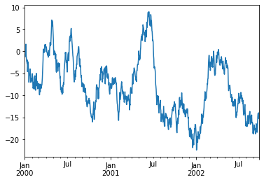
# Plotting Time Series
ts = pd.Series(np.random.randn(1000), index=pd.date_range("1/1/2000", periods=1000))

ts = ts.cumsum()

ts.plot()
<AxesSubplot:>
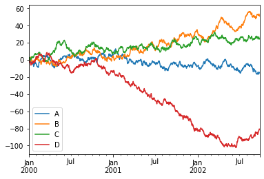
# Plotting DataFrame
df = pd.DataFrame(np.random.randn(1000, 4), index=ts.index, columns=["A", "B", "C", "D"])

df = df.cumsum()

plt.figure()

df.plot()

plt.legend(loc='best')
<matplotlib.legend.Legend at 0x216943bc190>


<Figure size 432x288 with 0 Axes>
statsmodels
statsmodels - https://www.statsmodels.org/stable/index.html#
- examples: https://www.statsmodels.org/stable/examples/index.html
The package statsmodels is a free software library for python including the following functions:
- Statistical models
- Hypothesis tests
- Data exploration
- Works in Python scripts, the Python and IPython shell and the jupyter notebook
%matplotlib inline
import numpy as np
import pandas as pd
import matplotlib.pyplot as plt

import statsmodels.api as sm

np.random.seed(9876789)
OLS estimation
# Artificial data:
nsample = 100
x = np.linspace(0, 10, 100)
X = np.column_stack((x, x**2))
beta = np.array([1, 0.1, 10])
e = np.random.normal(size=nsample)
# Our model needs an intercept so we add a column of 1s:
X = sm.add_constant(X)
y = np.dot(X, beta) + 100*e
# Fit and summary:
model = sm.OLS(y, X)
results = model.fit()
print(results.summary())
                            OLS Regression Results
==============================================================================
Dep. Variable:                      y   R-squared:                       0.887
Model:                            OLS   Adj. R-squared:                  0.884
Method:                 Least Squares   F-statistic:                     379.9
Date:                Wed, 10 Feb 2021   Prob (F-statistic):           1.30e-46
Time:                        17:30:51   Log-Likelihood:                -607.03
No. Observations:                 100   AIC:                             1220.
Df Residuals:                      97   BIC:                             1228.
Df Model:                           2
Covariance Type:            nonrobust
==============================================================================
                 coef    std err          t      P>|t|      [0.025      0.975]
------------------------------------------------------------------------------
const         35.2335     31.273      1.127      0.263     -26.834      97.301
x1           -13.9249     14.453     -0.963      0.338     -42.611      14.761
x2            11.0254      1.399      7.883      0.000       8.250      13.801
==============================================================================
Omnibus:                        2.042   Durbin-Watson:                   2.274
Prob(Omnibus):                  0.360   Jarque-Bera (JB):                1.875
Skew:                           0.234   Prob(JB):                        0.392
Kurtosis:                       2.519   Cond. No.                         144.
==============================================================================

Notes:
[1] Standard Errors assume that the covariance matrix of the errors is correctly specified.
matplotlib
matplotlib - https://matplotlib.org/
The package matplotlib is a free software library for python including the following functions:
- Image plots, Contour plots, Scatter plots, Polar plots, Line plots, 3D plots,
- Variety of hardcopy formats,
- Works in Python scripts, the Python and IPython shell and the jupyter notebook,
- Interactive environments.
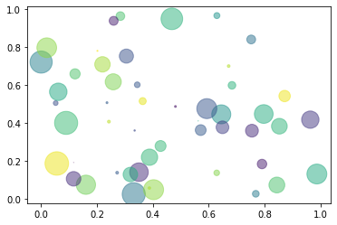
"""
simple demo of a scatter plot.
"""
import numpy as np
import matplotlib.pyplot as plt

N=50
x= np.random.rand(N)
y= np.random.rand(N)
colors= np.random.rand(N)
area = np.pi * (15 * np.random.rand(N))**2

plt.scatter(x,y, s=area, c=colors, alpha=0.5)
plt.show()
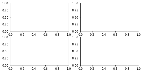
# create figures
fig = plt.figure(figsize=(8, 4))

# adding subplots
ax1 = fig.add_subplot(2, 2, 1)
ax2 = fig.add_subplot(2, 2, 2)
ax3 = fig.add_subplot(2, 2, 3)
ax4 = fig.add_subplot(2, 2, 4)
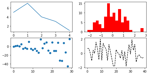
# Filling subplots with content
from numpy.random import randn
ax1.plot([5, 7, 4, 3, 1])
ax2.hist(randn(100), bins=20, color="r")
ax3.scatter(np.arange(30), np.arange(30) * randn(30))
ax4.plot(randn(40), "k--")
fig
Random number generators
https://docs.python.org/3/library/random.html
import random

def lottery():
    # returns 6 numbers between 1 and 40
    for i in range(6):
        yield random.randint(1, 40)

    # returns a 7th number between 1 and 15
    yield random.randint(1,15)

for random_number in lottery():
       print("And the next number is... %d!" %(random_number))
And the next number is... 2!
And the next number is... 9!
And the next number is... 3!
And the next number is... 22!
And the next number is... 12!
And the next number is... 22!
And the next number is... 4!
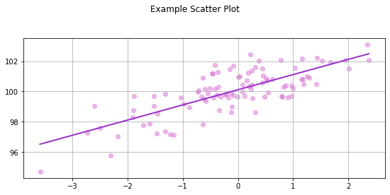
Plotting OLS
import numpy as np
import matplotlib.pyplot as plt
import statsmodels.api as sm

# numpy
x = np.random.randn(100)
y = x + np.random.randn(100) + 100

# matplotlib
fig, ax = plt.subplots(figsize=(8, 4))
ax.scatter(x, y, alpha=0.5, color='orchid')
fig.suptitle('Example Scatter Plot')
fig.tight_layout(pad=2);
ax.grid(True)

# statsmodels
x = sm.add_constant(x) # constant intercept term
# Model: y ~ x + c
model = sm.OLS(y, x)
fitted = model.fit()
x_pred = np.linspace(x.min(), x.max(), 50)
x_pred2 = sm.add_constant(x_pred)
y_pred = fitted.predict(x_pred2)

ax.plot(x_pred, y_pred, '-', color='darkorchid', linewidth=2)
[<matplotlib.lines.Line2D at 0x21694596a60>]