
Basic & Econometrics - Examples of feature engineering and cross-validation
Online Shoppers Intention Prediction
Sources:
http://archive.ics.uci.edu/ml/datasets/Online+Shoppers+Purchasing+Intention+Dataset https://github.com/zeglam/Online-shoppers-intention-prediction/blob/master/LICENSE
Data Description:
The dataset consists of feature vectors belonging to 12,330 sessions. The dataset was formed so that each session would belong to a different user in a 1-year period to avoid any tendency to a specific campaign, special day, user profile, or period. Of the 12,330 sessions in the dataset, 84.5% (10,422) were negative class samples that did not end with shopping, and the rest (1908) were positive class samples ending with shopping.
Numerical features
| Feature name | Feature description | Min. val | Max. val | SD | |:————-|:——————————————————————–|:———|:———|:——-| | Admin. | #pages visited by the visitor about account management | 0 | 27 | 3.32 | | Ad. duration | #seconds spent by the visitor on account management related pages | 0 | 3398 | 176.70 | | Info. | #informational pages visited by the visitor | 0 | 24 | 1.26 | | Info. durat. | #seconds spent by the visitor on informational pages | 0 | 2549 | 140.64 | | Prod. | #pages visited by visitor about product related pages | 0 | 705 | 44.45 | | Prod.durat. | #seconds spent by the visitor on product related pages | 0 | 63,973 | 1912.3 | | Bounce rate | Average bounce rate value of the pages visited by the visitor | 0 | 0.2 | 0.04 | | Exit rate | Average exit rate value of the pages visited by the visitor | 0 | 0.2 | 0.05 | | Page value | Average page value of the pages visited by the visitor | 0 | 361 | 18.55 | | Special day | Closeness of the site visiting time to a special day | 0 | 1.0 | 0.19 |
Categorical features
| Feature name | Feature description | Number of Values | |:——————–|:————————————————————————-|:—————–| | OperatingSystems | Operating system of the visitor | 8 | | Browser | Browser of the visitor | 13 | | Region | Geographic region from which the session has been started by the visitor | 9 | | TrafficType | Traffic source (e.g., banner, SMS, direct) | 20 | | VisitorType | Visitor type as “New Visitor,” “Returning Visitor,” and “Other” | 3 | | Weekend | Boolean value indicating whether the date of the visit is weekend | 2 | | Month | Month value of the visit date | 12 | | Revenue | Class label: whether the visit has been finalized with a transaction | 2 |
Project Goal
The main goal of this project is to design a machine learning classification system, that is able to predict an online shopper’s intention ( buy or no buy ), based on the values of the given features.
We will try a number of different classification algorithms, and compare their performance, in order to pick the best one for the project.
Libraries Import
import numpy as np
import pandas as pd

import seaborn as sns
import matplotlib.pyplot as plt
%matplotlib inline
plt.style.use('ggplot')

from sklearn.model_selection import train_test_split
from sklearn.preprocessing import StandardScaler
from sklearn import metrics
from sklearn.model_selection import GridSearchCV
from sklearn.model_selection import RandomizedSearchCV
from sklearn.model_selection import cross_val_score
from sklearn.metrics import confusion_matrix
from sklearn.metrics import roc_curve, auc
from sklearn.metrics import classification_report

from sklearn.naive_bayes import GaussianNB
from sklearn.neighbors import KNeighborsClassifier
from sklearn.svm import SVC
from sklearn.linear_model import LogisticRegression
from sklearn.ensemble import RandomForestClassifier
from sklearn.ensemble import GradientBoostingClassifier
from sklearn.ensemble import AdaBoostClassifier
from sklearn.tree import DecisionTreeClassifier
Data Import
df = pd.read_csv("../data/online_shoppers_intention.csv")
Data Description
Data Header
df.head(3)
| Administrative | Administrative_Duration | Informational | Informational_Duration | ProductRelated | ProductRelated_Duration | BounceRates | ExitRates | PageValues | SpecialDay | Month | OperatingSystems | Browser | Region | TrafficType | VisitorType | Weekend | Revenue | |
|---|---|---|---|---|---|---|---|---|---|---|---|---|---|---|---|---|---|---|
| 0 | 0 | 0.0 | 0 | 0.0 | 1 | 0.0 | 0.2 | 0.2 | 0.0 | 0.0 | Feb | 1 | 1 | 1 | 1 | Returning_Visitor | False | False |
| 1 | 0 | 0.0 | 0 | 0.0 | 2 | 64.0 | 0.0 | 0.1 | 0.0 | 0.0 | Feb | 2 | 2 | 1 | 2 | Returning_Visitor | False | False |
| 2 | 0 | 0.0 | 0 | 0.0 | 1 | 0.0 | 0.2 | 0.2 | 0.0 | 0.0 | Feb | 4 | 1 | 9 | 3 | Returning_Visitor | False | False |
Data Types
df.info()
<class 'pandas.core.frame.DataFrame'>
RangeIndex: 12330 entries, 0 to 12329
Data columns (total 18 columns):
 #   Column                   Non-Null Count  Dtype
---  ------                   --------------  -----
 0   Administrative           12330 non-null  int64
 1   Administrative_Duration  12330 non-null  float64
 2   Informational            12330 non-null  int64
 3   Informational_Duration   12330 non-null  float64
 4   ProductRelated           12330 non-null  int64
 5   ProductRelated_Duration  12330 non-null  float64
 6   BounceRates              12330 non-null  float64
 7   ExitRates                12330 non-null  float64
 8   PageValues               12330 non-null  float64
 9   SpecialDay               12330 non-null  float64
 10  Month                    12330 non-null  object
 11  OperatingSystems         12330 non-null  int64
 12  Browser                  12330 non-null  int64
 13  Region                   12330 non-null  int64
 14  TrafficType              12330 non-null  int64
 15  VisitorType              12330 non-null  object
 16  Weekend                  12330 non-null  bool
 17  Revenue                  12330 non-null  bool
dtypes: bool(2), float64(7), int64(7), object(2)
memory usage: 1.5+ MB
Here we can see that most of our dataset is numerical, either integers or floats; Revenue and Weekend are boolean type, and they can easly be transformed into binary type (0 & 1).
Statistical Analysis of Our Dataset
df.describe()
| Administrative | Administrative_Duration | Informational | Informational_Duration | ProductRelated | ProductRelated_Duration | BounceRates | ExitRates | PageValues | SpecialDay | OperatingSystems | Browser | Region | TrafficType | |
|---|---|---|---|---|---|---|---|---|---|---|---|---|---|---|
| count | 12330.000000 | 12330.000000 | 12330.000000 | 12330.000000 | 12330.000000 | 12330.000000 | 12330.000000 | 12330.000000 | 12330.000000 | 12330.000000 | 12330.000000 | 12330.000000 | 12330.000000 | 12330.000000 |
| mean | 2.315166 | 80.818611 | 0.503569 | 34.472398 | 31.731468 | 1194.746220 | 0.022191 | 0.043073 | 5.889258 | 0.061427 | 2.124006 | 2.357097 | 3.147364 | 4.069586 |
| std | 3.321784 | 176.779107 | 1.270156 | 140.749294 | 44.475503 | 1913.669288 | 0.048488 | 0.048597 | 18.568437 | 0.198917 | 0.911325 | 1.717277 | 2.401591 | 4.025169 |
| min | 0.000000 | 0.000000 | 0.000000 | 0.000000 | 0.000000 | 0.000000 | 0.000000 | 0.000000 | 0.000000 | 0.000000 | 1.000000 | 1.000000 | 1.000000 | 1.000000 |
| 25% | 0.000000 | 0.000000 | 0.000000 | 0.000000 | 7.000000 | 184.137500 | 0.000000 | 0.014286 | 0.000000 | 0.000000 | 2.000000 | 2.000000 | 1.000000 | 2.000000 |
| 50% | 1.000000 | 7.500000 | 0.000000 | 0.000000 | 18.000000 | 598.936905 | 0.003112 | 0.025156 | 0.000000 | 0.000000 | 2.000000 | 2.000000 | 3.000000 | 2.000000 |
| 75% | 4.000000 | 93.256250 | 0.000000 | 0.000000 | 38.000000 | 1464.157213 | 0.016813 | 0.050000 | 0.000000 | 0.000000 | 3.000000 | 2.000000 | 4.000000 | 4.000000 |
| max | 27.000000 | 3398.750000 | 24.000000 | 2549.375000 | 705.000000 | 63973.522230 | 0.200000 | 0.200000 | 361.763742 | 1.000000 | 8.000000 | 13.000000 | 9.000000 | 20.000000 |
Data Cleaning
Missing Data Points
print(df.isnull().sum())
Administrative             0
Administrative_Duration    0
Informational              0
Informational_Duration     0
ProductRelated             0
ProductRelated_Duration    0
BounceRates                0
ExitRates                  0
PageValues                 0
SpecialDay                 0
Month                      0
OperatingSystems           0
Browser                    0
Region                     0
TrafficType                0
VisitorType                0
Weekend                    0
Revenue                    0
dtype: int64
It looks like our dataset has no missing values at all, which is great.
Data Type Fix
We will transform Revenue & Weekend features from boolean into binary, so that we can easily use them in our later calculations.
df.Revenue = df.Revenue.astype('int')
df.Weekend = df.Weekend.astype('int')
Now, let’s check dataset info:
df.info()
<class 'pandas.core.frame.DataFrame'>
RangeIndex: 12330 entries, 0 to 12329
Data columns (total 18 columns):
 #   Column                   Non-Null Count  Dtype
---  ------                   --------------  -----
 0   Administrative           12330 non-null  int64
 1   Administrative_Duration  12330 non-null  float64
 2   Informational            12330 non-null  int64
 3   Informational_Duration   12330 non-null  float64
 4   ProductRelated           12330 non-null  int64
 5   ProductRelated_Duration  12330 non-null  float64
 6   BounceRates              12330 non-null  float64
 7   ExitRates                12330 non-null  float64
 8   PageValues               12330 non-null  float64
 9   SpecialDay               12330 non-null  float64
 10  Month                    12330 non-null  object
 11  OperatingSystems         12330 non-null  int64
 12  Browser                  12330 non-null  int64
 13  Region                   12330 non-null  int64
 14  TrafficType              12330 non-null  int64
 15  VisitorType              12330 non-null  object
 16  Weekend                  12330 non-null  int64
 17  Revenue                  12330 non-null  int64
dtypes: float64(7), int64(9), object(2)
memory usage: 1.7+ MB
Both Revenue and Weekend has been transformed into binary (0’s and 1’s).
EDA
Correlation Analysis
matrix = np.triu(df.corr())
fig, ax = plt.subplots(figsize=(12,12))
sns.heatmap(df.corr(), annot=True, ax=ax, fmt='.1g', vmin=-1, vmax=1, center= 0, mask=matrix, cmap='RdBu_r')
plt.show()
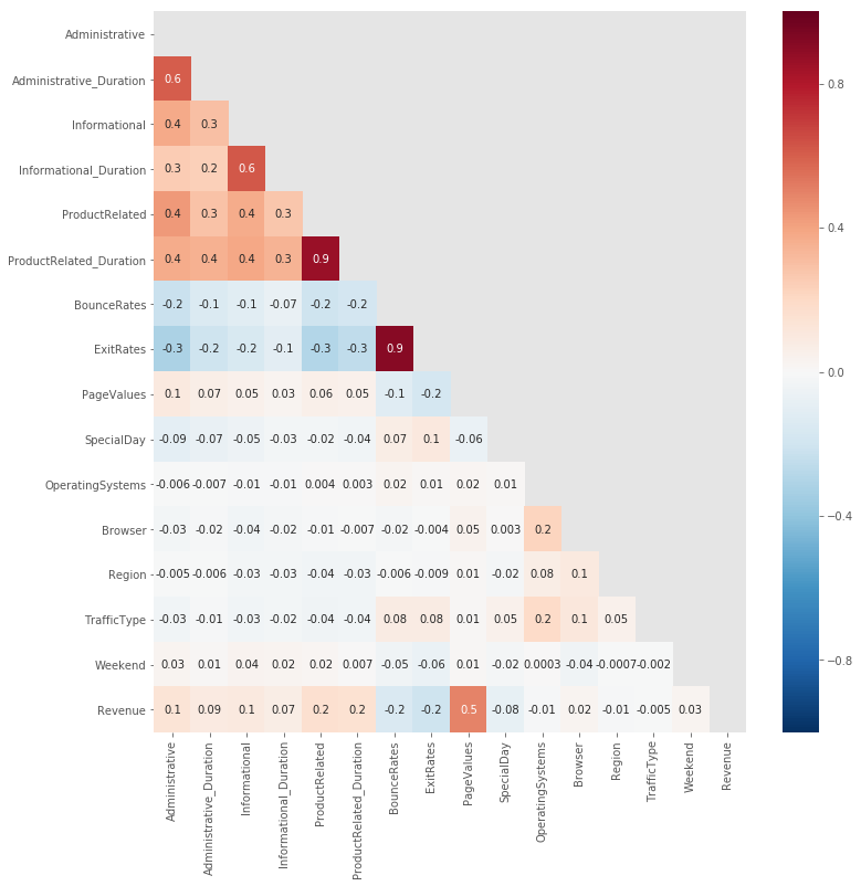
From the above heatmap, we observe the following:
- In general, there is very little correlation among the different features in our dataset.
-
The very few cases of high correlation ( corr >= 0.7) are: - BounceRates & ExitRates (0.9).
- ProductRelated & ProductRelated_Duration (0.9).
-
Moderate Correlations (0.3 < corr < 0.7): - Among the following features: Administrative, Administrative_Duration, Informational, Informational_Duration, ProductRelated, and ProductRelated_Duration.
- Also between PageValues and Revenue.
let’s now show correlation among a few of our features
g1 = sns.pairplot(df[['Administrative', 'Informational', 'ProductRelated', 'PageValues', 'Revenue']], hue='Revenue')
g1.fig.suptitle('Feature Relations')
plt.show()
/Users/manguito/.virtualenvs/myEnv/lib/python3.7/site-packages/scipy/stats/stats.py:1713: FutureWarning: Using a non-tuple sequence for multidimensional indexing is deprecated; use `arr[tuple(seq)]` instead of `arr[seq]`. In the future this will be interpreted as an array index, `arr[np.array(seq)]`, which will result either in an error or a different result.
  return np.add.reduce(sorted[indexer] * weights, axis=axis) / sumval
/Users/manguito/.virtualenvs/myEnv/lib/python3.7/site-packages/statsmodels/nonparametric/kde.py:488: RuntimeWarning: invalid value encountered in true_divide
  binned = fast_linbin(X, a, b, gridsize) / (delta * nobs)
/Users/manguito/.virtualenvs/myEnv/lib/python3.7/site-packages/statsmodels/nonparametric/kdetools.py:34: RuntimeWarning: invalid value encountered in double_scalars
  FAC1 = 2*(np.pi*bw/RANGE)**2
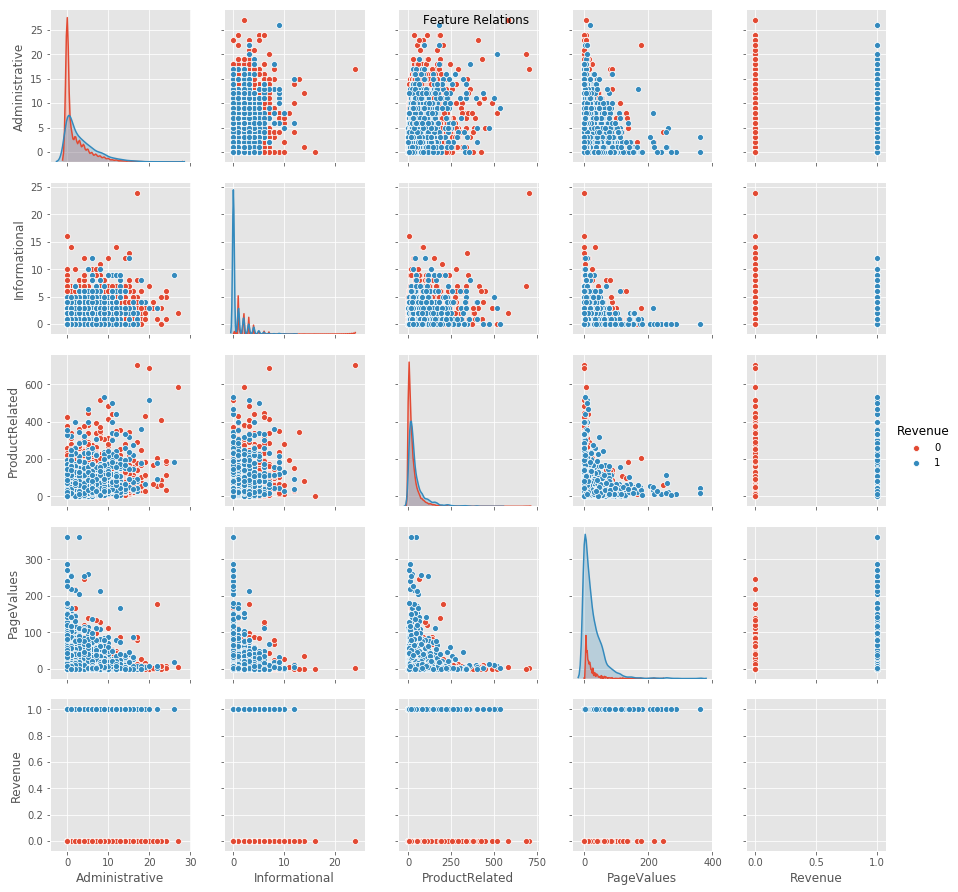
From the above figure, we can see:
- No strong correlation between Revenue (our target) and any other feature.
- A strong negative correlation between PageValues and other features shown.
Web Pages Analysis
fig = plt.figure(figsize=(12, 12))

ax1 = fig.add_subplot(2, 3, 1)
ax2 = fig.add_subplot(2, 3, 2)
ax3 = fig.add_subplot(2, 3, 3)
ax4 = fig.add_subplot(2, 3, 4)
ax5 = fig.add_subplot(2, 3, 5)
ax6 = fig.add_subplot(2, 3, 6)

sns.violinplot(data=df, x = 'Revenue', y = 'Administrative', ax=ax1)
sns.violinplot(data=df, x = 'Revenue', y = 'Informational', ax=ax2)
sns.violinplot(data=df, x = 'Revenue', y = 'ProductRelated', ax=ax3)
sns.boxplot(data=df, x = 'Revenue', y = 'Administrative_Duration', ax=ax4)
sns.boxplot(data=df, x = 'Revenue', y = 'Informational_Duration', ax=ax5)
sns.boxplot(data=df, x = 'Revenue', y = 'ProductRelated_Duration', ax=ax6)

plt.tight_layout()
plt.show()
/Users/manguito/.virtualenvs/myEnv/lib/python3.7/site-packages/scipy/stats/stats.py:1713: FutureWarning: Using a non-tuple sequence for multidimensional indexing is deprecated; use `arr[tuple(seq)]` instead of `arr[seq]`. In the future this will be interpreted as an array index, `arr[np.array(seq)]`, which will result either in an error or a different result.
  return np.add.reduce(sorted[indexer] * weights, axis=axis) / sumval
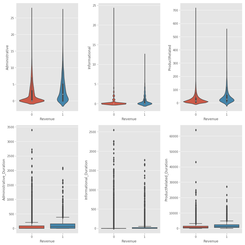
From the above boxplots, we can see that:
- In general, visitors tend to visit less pages, and spend less time, if they are not going to make a purchase.
- The number of product related pages, and the time spent on them, is way higher than that for account related or informational pages.
- The first 3 feature look like they follow a skewed normal distribution.
Page Metrics Analysis
fig = plt.figure(figsize=(16, 4))

ax1 = fig.add_subplot(1, 3, 1)
ax2 = fig.add_subplot(1, 3, 2)
ax3 = fig.add_subplot(1, 3, 3)

sns.distplot(df['BounceRates'], bins=20, ax=ax1)
sns.distplot(df['ExitRates'], bins=20, ax=ax2)
sns.distplot(df['PageValues'], bins=20, ax=ax3)

plt.tight_layout()
plt.show()
/Users/manguito/.virtualenvs/myEnv/lib/python3.7/site-packages/scipy/stats/stats.py:1713: FutureWarning: Using a non-tuple sequence for multidimensional indexing is deprecated; use `arr[tuple(seq)]` instead of `arr[seq]`. In the future this will be interpreted as an array index, `arr[np.array(seq)]`, which will result either in an error or a different result.
  return np.add.reduce(sorted[indexer] * weights, axis=axis) / sumval
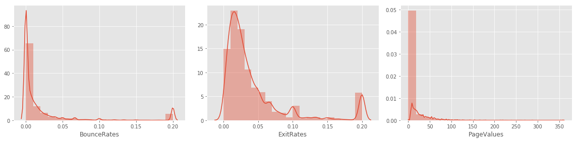
From the above visualizations of 3 google analytics metrics, we can conclude:
- BounceRates & PageValues do not follow a normal distribution.
- All 3 features have distributions that are skewed right.
- All 3 distributions have a lot of outliers.
- The average bounce and exit rates of most of our data points is low, which is good, since high rates identicate that visitors are not engaging with the website.
- Exit rate has more high values than bounce rate, which makes sense, where transaction confirmation pages for example will cause the average exit rate to increase.
- Bounce rate ==> the percentage where the first page visited was the only page visited in that session.
- Exit rate of a page ==> The percentage where that page was the last page visited in the session, out of all visits to that page.
Visitor Analysis
fig = plt.figure(figsize=(18, 6))

ax1 = fig.add_subplot(2, 2, 1)
ax2 = fig.add_subplot(2, 2, 2)
ax3 = fig.add_subplot(2, 2, 3)
ax4 = fig.add_subplot(2, 2, 4)

sns.countplot(data=df, x='OperatingSystems', hue='VisitorType', ax=ax1)
sns.countplot(data=df, x='Browser', hue='VisitorType', ax=ax2)
sns.countplot(data=df, x='Region', hue='VisitorType', ax=ax3)
sns.countplot(data=df, x='TrafficType', hue='VisitorType', ax=ax4)

ax1.legend(loc='upper right')
ax2.legend(loc='upper right')
ax3.legend(loc='upper right')
ax4.legend(loc='upper right')
plt.tight_layout()
plt.show()
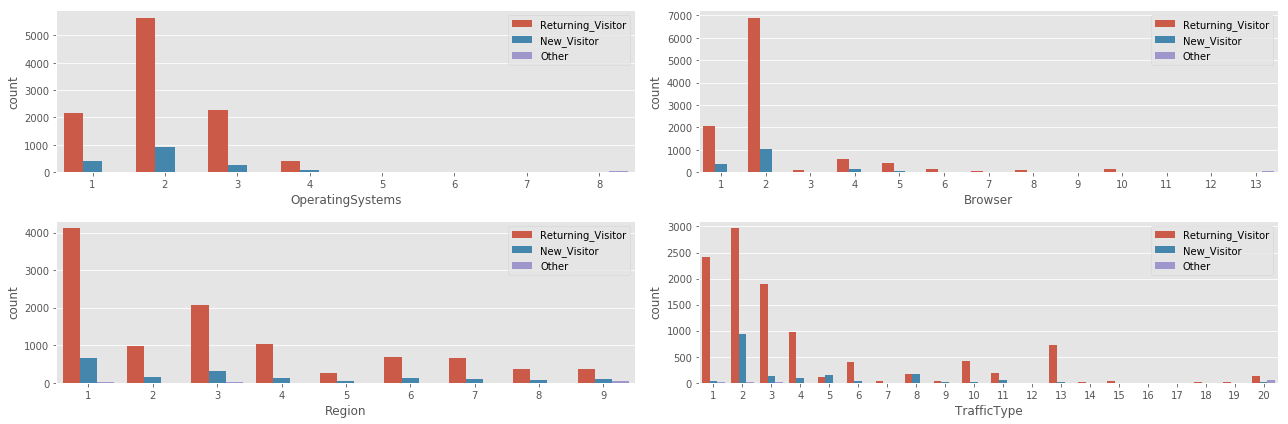
- 1 Operating system is responsible for ~7000 of the examples in our dataset.
- 4 of the 8 operating systems used, are responsible of a very small number (<200) of the examples in our dataset.
- A similar story repeated with the browsers used by visitors, where there is 1 dominant browser, 3 with decent representation in the dataset, and the rest are rarey used.
- It looks like we have a very regionally diverse traffic in our dataset.
- Also Traffic sources are very diverse, with a few that did not contribute much to the dataset.
Visit Date Analysis
fig = plt.figure(figsize=(18, 12))
ax1 = fig.add_subplot(2, 1, 1)
ax2 = fig.add_subplot(2, 1, 2)
orderlist = ['Jan','Feb','Mar','Apr','May','June','Jul','Aug','Sep','Oct','Nov','Dec']
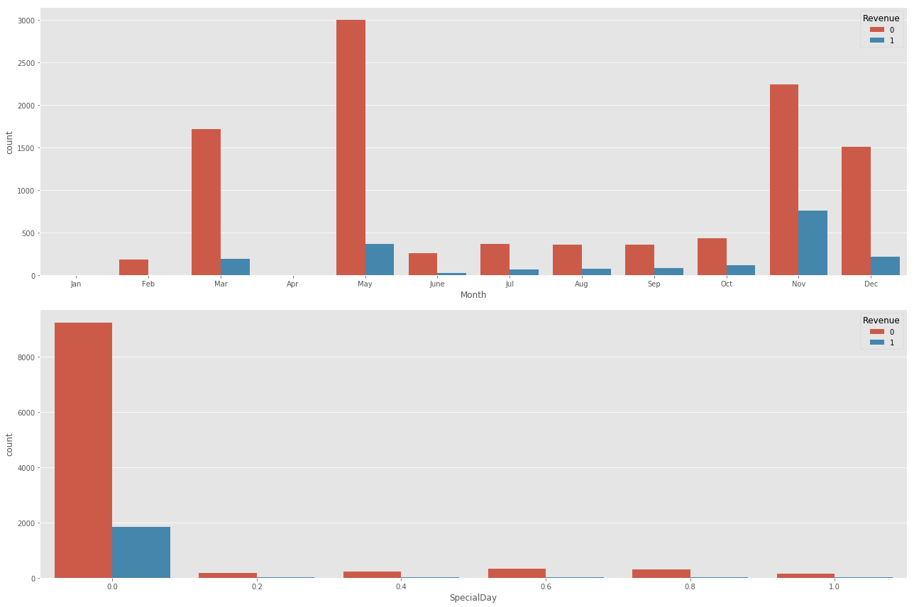
sns.countplot(data=df, x='Month', hue='Revenue', ax=ax1, order=orderlist)
sns.countplot(data=df, x='SpecialDay', hue='Revenue', ax=ax2)
plt.tight_layout()
plt.show()
fig, ax = plt.subplots(1, 2,figsize=(12, 6), subplot_kw=dict(aspect="equal"))
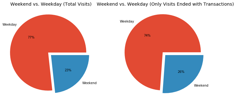
ax[0].pie(df['Weekend'].value_counts(),explode=(0.1,0),labels=['Weekday','Weekend'], autopct='%1.0f%%')
ax[0].set_title('Weekend vs. Weekday (Total Visits)')
ax[1].pie(df[df['Revenue'] == 1]['Weekend'].value_counts(),explode=(0.1,0),labels=['Weekday','Weekend'], autopct='%1.0f%%')
ax[1].set_title('Weekend vs. Weekday (Only Visits Ended with Transactions)')
#fig.suptitle('Weekend Visits')
plt.show()
- On March and May, we have a lot of visits (May is the month with the highest number of visits), yet transactions made during those 2 months are not on the same level.
- We have no visits at all during Jan nor Apr.
- Most transactions happen during the end of the year, with Nov as the month with the highest number of confirmed transactions.
- The closer the visit date to a special day (like black Friday, new year’s, … etc) the more likely it will end up in a transaction.
- Most of transactions happen on special days (SpecialDay =0).
- It does not look like weekends affect the number of visits or transactions much, we can see only a slight increase in the number of transactions happening on weekends compared to those on weekdays.
Data Pre-Processing
In this section we will make our data ready for model training. This will include:
- Transform Month and VisitorType columns into numerical (binary) values.
- Split data set into training, validation, and testing parts (70/15/15), while separating Revenue column, where it will be used as our labels.
- We will ably feature scaling on our input data, in order to be used for Naive Bayes and SVM model training.
Data Transformation
dff = pd.concat([df,pd.get_dummies(df['Month'], prefix='Month')], axis=1).drop(['Month'],axis=1)
dff = pd.concat([dff,pd.get_dummies(dff['VisitorType'], prefix='VisitorType')], axis=1).drop(['VisitorType'],axis=1)
print(dff.info())
<class 'pandas.core.frame.DataFrame'>
RangeIndex: 12330 entries, 0 to 12329
Data columns (total 29 columns):
 #   Column                         Non-Null Count  Dtype
---  ------                         --------------  -----
 0   Administrative                 12330 non-null  int64
 1   Administrative_Duration        12330 non-null  float64
 2   Informational                  12330 non-null  int64
 3   Informational_Duration         12330 non-null  float64
 4   ProductRelated                 12330 non-null  int64
 5   ProductRelated_Duration        12330 non-null  float64
 6   BounceRates                    12330 non-null  float64
 7   ExitRates                      12330 non-null  float64
 8   PageValues                     12330 non-null  float64
 9   SpecialDay                     12330 non-null  float64
 10  OperatingSystems               12330 non-null  int64
 11  Browser                        12330 non-null  int64
 12  Region                         12330 non-null  int64
 13  TrafficType                    12330 non-null  int64
 14  Weekend                        12330 non-null  int64
 15  Revenue                        12330 non-null  int64
 16  Month_Aug                      12330 non-null  uint8
 17  Month_Dec                      12330 non-null  uint8
 18  Month_Feb                      12330 non-null  uint8
 19  Month_Jul                      12330 non-null  uint8
 20  Month_June                     12330 non-null  uint8
 21  Month_Mar                      12330 non-null  uint8
 22  Month_May                      12330 non-null  uint8
 23  Month_Nov                      12330 non-null  uint8
 24  Month_Oct                      12330 non-null  uint8
 25  Month_Sep                      12330 non-null  uint8
 26  VisitorType_New_Visitor        12330 non-null  uint8
 27  VisitorType_Other              12330 non-null  uint8
 28  VisitorType_Returning_Visitor  12330 non-null  uint8
dtypes: float64(7), int64(9), uint8(13)
memory usage: 1.7 MB
None
dff.head()
| Administrative | Administrative_Duration | Informational | Informational_Duration | ProductRelated | ProductRelated_Duration | BounceRates | ExitRates | PageValues | SpecialDay | ... | Month_Jul | Month_June | Month_Mar | Month_May | Month_Nov | Month_Oct | Month_Sep | VisitorType_New_Visitor | VisitorType_Other | VisitorType_Returning_Visitor | |
|---|---|---|---|---|---|---|---|---|---|---|---|---|---|---|---|---|---|---|---|---|---|
| 0 | 0 | 0.0 | 0 | 0.0 | 1 | 0.000000 | 0.20 | 0.20 | 0.0 | 0.0 | ... | 0 | 0 | 0 | 0 | 0 | 0 | 0 | 0 | 0 | 1 |
| 1 | 0 | 0.0 | 0 | 0.0 | 2 | 64.000000 | 0.00 | 0.10 | 0.0 | 0.0 | ... | 0 | 0 | 0 | 0 | 0 | 0 | 0 | 0 | 0 | 1 |
| 2 | 0 | 0.0 | 0 | 0.0 | 1 | 0.000000 | 0.20 | 0.20 | 0.0 | 0.0 | ... | 0 | 0 | 0 | 0 | 0 | 0 | 0 | 0 | 0 | 1 |
| 3 | 0 | 0.0 | 0 | 0.0 | 2 | 2.666667 | 0.05 | 0.14 | 0.0 | 0.0 | ... | 0 | 0 | 0 | 0 | 0 | 0 | 0 | 0 | 0 | 1 |
| 4 | 0 | 0.0 | 0 | 0.0 | 10 | 627.500000 | 0.02 | 0.05 | 0.0 | 0.0 | ... | 0 | 0 | 0 | 0 | 0 | 0 | 0 | 0 | 0 | 1 |
5 rows × 29 columns
Data Split
y = dff['Revenue']
X = dff.drop(['Revenue'], axis=1)
len(y)
12330
X_train, X_valtest, y_train, y_valtest = train_test_split(X, y, test_size=0.3, random_state=101)
X_val, X_test, y_val, y_test = train_test_split(X_valtest, y_valtest, test_size=0.5, random_state=101)
Now we have the following data subsets:
- Train data (X_train) and trin labels (y_train) ==> 70%
- Validation data (X_val) and validation labels (y_val) ==> 15%
- Test data (X_test) and test labels (y)test) ==> 15%
Data Scaling
We will scale the features in our subsets, in order to use them to train, validate, and test models that will benefit from feature scaling.
sc_X = StandardScaler()

Xsc_train = sc_X.fit_transform(X_train)
Xsc_val = sc_X.fit_transform(X_val)
Xsc_test = sc_X.fit_transform(X_test)
/Users/manguito/.virtualenvs/myEnv/lib/python3.7/site-packages/sklearn/preprocessing/data.py:645: DataConversionWarning: Data with input dtype uint8, int64, float64 were all converted to float64 by StandardScaler.
  return self.partial_fit(X, y)
/Users/manguito/.virtualenvs/myEnv/lib/python3.7/site-packages/sklearn/base.py:464: DataConversionWarning: Data with input dtype uint8, int64, float64 were all converted to float64 by StandardScaler.
  return self.fit(X, **fit_params).transform(X)
Model Building
Logistic Regression
lrm = LogisticRegression(C=1.0,solver='lbfgs',max_iter=10000) #default parameters
lrm.fit(X_train,y_train)
lrm_pred = lrm.predict(X_val)

print('Logistic Regression initial Performance:')
print('----------------------------------------')
print('Accuracy        : ', metrics.accuracy_score(y_val, lrm_pred))
print('F1 Score        : ', metrics.f1_score(y_val, lrm_pred))
print('Precision       : ', metrics.precision_score(y_val, lrm_pred))
print('Recall          : ', metrics.recall_score(y_val, lrm_pred))
print('Confusion Matrix:\n ', confusion_matrix(y_val, lrm_pred))
Logistic Regression initial Performance:
----------------------------------------
Accuracy        :  0.8783126014061655
F1 Score        :  0.5243128964059196
Precision       :  0.7515151515151515
Recall          :  0.4025974025974026
Confusion Matrix:
  [[1500   41]
 [ 184  124]]
K-fold Cross-Validation
https://scikit-learn.org/stable/auto_examples/model_selection/plot_cv_indices.html#sphx-glr-auto-examples-model-selection-plot-cv-indices-py
from sklearn.model_selection import (TimeSeriesSplit, KFold, ShuffleSplit,
                                     StratifiedKFold, GroupShuffleSplit,
                                     GroupKFold, StratifiedShuffleSplit)
from matplotlib.patches import Patch
np.random.seed(1338)
cmap_data = plt.cm.Paired
cmap_cv = plt.cm.coolwarm
n_splits = 4
Split data into train and test data
X_train, X_test, y_train, y_test = train_test_split(X, y, test_size=0.3, random_state=101)
Xsc_train = sc_X.fit_transform(X_train)
Xsc_test = sc_X.fit_transform(X_test)

Xsc_train_df = pd.DataFrame(Xsc_train, index=X_train.index, columns=X_train.columns)
Xsc_test_df = pd.DataFrame(Xsc_test, index=X_test.index, columns=X_test.columns)
/Users/manguito/.virtualenvs/myEnv/lib/python3.7/site-packages/sklearn/preprocessing/data.py:645: DataConversionWarning: Data with input dtype uint8, int64, float64 were all converted to float64 by StandardScaler.
  return self.partial_fit(X, y)
/Users/manguito/.virtualenvs/myEnv/lib/python3.7/site-packages/sklearn/base.py:464: DataConversionWarning: Data with input dtype uint8, int64, float64 were all converted to float64 by StandardScaler.
  return self.fit(X, **fit_params).transform(X)
X_train.head()
| Administrative | Administrative_Duration | Informational | Informational_Duration | ProductRelated | ProductRelated_Duration | BounceRates | ExitRates | PageValues | SpecialDay | ... | Month_Jul | Month_June | Month_Mar | Month_May | Month_Nov | Month_Oct | Month_Sep | VisitorType_New_Visitor | VisitorType_Other | VisitorType_Returning_Visitor | |
|---|---|---|---|---|---|---|---|---|---|---|---|---|---|---|---|---|---|---|---|---|---|
| 7821 | 6 | 105.633333 | 2 | 105.95 | 8 | 246.386508 | 0.000000 | 0.008929 | 0.000000 | 0.0 | ... | 0 | 0 | 0 | 0 | 1 | 0 | 0 | 0 | 0 | 1 |
| 6701 | 0 | 0.000000 | 0 | 0.00 | 14 | 317.066667 | 0.035714 | 0.050000 | 0.000000 | 0.0 | ... | 0 | 0 | 0 | 0 | 0 | 0 | 0 | 0 | 0 | 1 |
| 11312 | 1 | 21.250000 | 0 | 0.00 | 92 | 2716.519048 | 0.006738 | 0.037885 | 23.738911 | 0.0 | ... | 0 | 0 | 0 | 0 | 1 | 0 | 0 | 0 | 0 | 1 |
| 3873 | 0 | 0.000000 | 0 | 0.00 | 7 | 203.666667 | 0.000000 | 0.009524 | 0.000000 | 0.0 | ... | 0 | 0 | 0 | 1 | 0 | 0 | 0 | 0 | 0 | 1 |
| 9319 | 1 | 14.000000 | 0 | 0.00 | 50 | 1317.795833 | 0.010000 | 0.021470 | 0.000000 | 0.0 | ... | 0 | 0 | 0 | 0 | 1 | 0 | 0 | 0 | 0 | 1 |
5 rows × 28 columns
Xsc_train_df.head()
| Administrative | Administrative_Duration | Informational | Informational_Duration | ProductRelated | ProductRelated_Duration | BounceRates | ExitRates | PageValues | SpecialDay | ... | Month_Jul | Month_June | Month_Mar | Month_May | Month_Nov | Month_Oct | Month_Sep | VisitorType_New_Visitor | VisitorType_Other | VisitorType_Returning_Visitor | |
|---|---|---|---|---|---|---|---|---|---|---|---|---|---|---|---|---|---|---|---|---|---|
| 7821 | 1.131955 | 0.156268 | 1.186984 | 0.530696 | -0.536100 | -0.517481 | -0.458955 | -0.704386 | -0.309198 | -0.307883 | ... | -0.192693 | -0.152435 | -0.426241 | -0.614893 | 1.762410 | -0.213717 | -0.197492 | -0.396978 | -0.078604 | 0.407282 |
| 6701 | -0.696588 | -0.460087 | -0.392550 | -0.246800 | -0.398929 | -0.478028 | 0.279525 | 0.142770 | -0.309198 | -0.307883 | ... | -0.192693 | -0.152435 | -0.426241 | -0.614893 | -0.567405 | -0.213717 | -0.197492 | -0.396978 | -0.078604 | 0.407282 |
| 11312 | -0.391831 | -0.336096 | -0.392550 | -0.246800 | 1.384297 | 0.861314 | -0.319639 | -0.107113 | 0.951488 | -0.307883 | ... | -0.192693 | -0.152435 | -0.426241 | -0.614893 | 1.762410 | -0.213717 | -0.197492 | -0.396978 | -0.078604 | 0.407282 |
| 3873 | -0.696588 | -0.460087 | -0.392550 | -0.246800 | -0.558962 | -0.541327 | -0.458955 | -0.692108 | -0.309198 | -0.307883 | ... | -0.192693 | -0.152435 | -0.426241 | 1.626299 | -0.567405 | -0.213717 | -0.197492 | -0.396978 | -0.078604 | 0.407282 |
| 9319 | -0.391831 | -0.378399 | -0.392550 | -0.246800 | 0.424098 | 0.080565 | -0.252181 | -0.445712 | -0.309198 | -0.307883 | ... | -0.192693 | -0.152435 | -0.426241 | -0.614893 | 1.762410 | -0.213717 | -0.197492 | -0.396978 | -0.078604 | 0.407282 |
5 rows × 28 columns
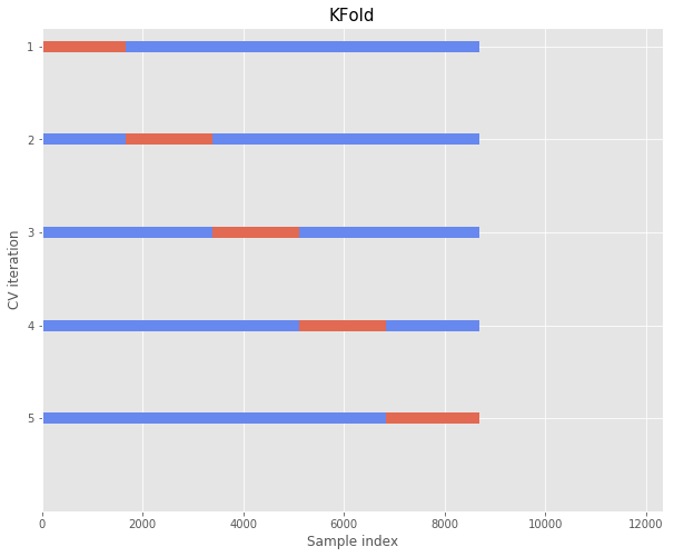
n_splits = 5


fig, ax = plt.subplots(figsize = (10,8))
cv = KFold(n_splits)
for ii, (tr, tt) in enumerate(cv.split(X=X_train, y=y_train)):
    # Fill in indices with the training/test groups
    indices = np.array([np.nan] * len(X))
    indices[tt] = 1
    indices[tr] = 0
    ax.scatter(range(len(indices)), [ii ] * len(indices),
                   c=indices, marker='_', lw=10, cmap=cmap_cv,
                   vmin=-.2, vmax=1.2)
    yticklabels = [i+1 for i in list(range(n_splits))]
    ax.set(yticks=np.arange(n_splits), yticklabels=yticklabels,
           xlabel='Sample index', ylabel="CV iteration",
           ylim=[n_splits, -.2], xlim=[0, len(y)])
    ax.set_title('{}'.format(type(cv).__name__), fontsize=15)
Compare accuracy of logistic regression and KNN
Note that we need to use scaled variables for KNN
logStats = {}
knnStats = {}
for ii, (tr, tt) in enumerate(cv.split(X=X_train, y=y_train)):
    # Fill in indices with the training/test groups
    indices = np.array([np.nan] * len(X))
    indices[tt] = 1
    indices[tr] = 0
# train Logistic Regression Model
    lrm = LogisticRegression(C=1.0,solver='lbfgs',max_iter=10000) #default parameters
    lrm.fit(X_train.iloc[tr,:],y_train.iloc[tr])
    lrm_pred = lrm.predict(X_train.iloc[tt,:])
    y_val = y_train.iloc[tt]

    print('Logistic Regression initial Performance:')
    print('----------------------------------------')
    print('Accuracy        : ', metrics.accuracy_score(y_val, lrm_pred))
    print('F1 Score        : ', metrics.f1_score(y_val, lrm_pred))
    print('Precision       : ', metrics.precision_score(y_val, lrm_pred))
    print('Recall          : ', metrics.recall_score(y_val, lrm_pred))
    print('Confusion Matrix:\n ', confusion_matrix(y_val, lrm_pred))
    logStats.setdefault('accuracy', []).append(metrics.accuracy_score(y_val, lrm_pred))

    knn = KNeighborsClassifier(n_neighbors=5,weights='uniform',leaf_size=30,p=2) #default values
    knn.fit(Xsc_train_df.iloc[tr,:],y_train.iloc[tr])
    knn_pred = knn.predict(Xsc_train_df.iloc[tt,:])

    print('K-Nearest Neighbor Initial Performance:')
    print('---------------------------------------')
    print('Accuracy        : ', metrics.accuracy_score(y_val, knn_pred))
    print('F1 Score        : ', metrics.f1_score(y_val, knn_pred))
    print('Precision       : ', metrics.precision_score(y_val, knn_pred))
    print('Recall          : ', metrics.recall_score(y_val, knn_pred))
    print('Confusion Matrix:\n ', confusion_matrix(y_val, knn_pred))
    knnStats.setdefault('accuracy', []).append(metrics.accuracy_score(y_val, knn_pred))
Logistic Regression initial Performance:
----------------------------------------
Accuracy        :  0.8726114649681529
F1 Score        :  0.45544554455445546
Precision       :  0.773109243697479
Recall          :  0.32280701754385965
Confusion Matrix:
  [[1415   27]
 [ 193   92]]
K-Nearest Neighbor Initial Performance:
---------------------------------------
Accuracy        :  0.8581354950781702
F1 Score        :  0.40389294403892945
Precision       :  0.6587301587301587
Recall          :  0.2912280701754386
Confusion Matrix:
  [[1399   43]
 [ 202   83]]
Logistic Regression initial Performance:
----------------------------------------
Accuracy        :  0.8823870220162224
F1 Score        :  0.5012285012285012
Precision       :  0.7338129496402878
Recall          :  0.3805970149253731
Confusion Matrix:
  [[1421   37]
 [ 166  102]]
K-Nearest Neighbor Initial Performance:
---------------------------------------
Accuracy        :  0.8742757821552724
F1 Score        :  0.4668304668304668
Precision       :  0.6834532374100719
Recall          :  0.35447761194029853
Confusion Matrix:
  [[1414   44]
 [ 173   95]]
Logistic Regression initial Performance:
----------------------------------------
Accuracy        :  0.8818076477404403
F1 Score        :  0.5
Precision       :  0.7445255474452555
Recall          :  0.3763837638376384
Confusion Matrix:
  [[1420   35]
 [ 169  102]]
K-Nearest Neighbor Initial Performance:
---------------------------------------
Accuracy        :  0.8719582850521437
F1 Score        :  0.45161290322580644
Precision       :  0.6893939393939394
Recall          :  0.33579335793357934
Confusion Matrix:
  [[1414   41]
 [ 180   91]]
Logistic Regression initial Performance:
----------------------------------------
Accuracy        :  0.8939745075318656
F1 Score        :  0.5040650406504066
Precision       :  0.7322834645669292
Recall          :  0.384297520661157
Confusion Matrix:
  [[1450   34]
 [ 149   93]]
K-Nearest Neighbor Initial Performance:
---------------------------------------
Accuracy        :  0.8765932792584009
F1 Score        :  0.4132231404958678
Precision       :  0.6198347107438017
Recall          :  0.30991735537190085
Confusion Matrix:
  [[1438   46]
 [ 167   75]]
Logistic Regression initial Performance:
----------------------------------------
Accuracy        :  0.8783314020857474
F1 Score        :  0.5047169811320754
Precision       :  0.7039473684210527
Recall          :  0.39338235294117646
Confusion Matrix:
  [[1409   45]
 [ 165  107]]
K-Nearest Neighbor Initial Performance:
---------------------------------------
Accuracy        :  0.8725376593279258
F1 Score        :  0.4634146341463415
Precision       :  0.6884057971014492
Recall          :  0.3492647058823529
Confusion Matrix:
  [[1411   43]
 [ 177   95]]
np.mean(logStats['accuracy']),np.mean(knnStats['accuracy'])
(0.8818224088684857, 0.8707001001743826)