
Basic & Econometrics - ARCH and GARCH modeling
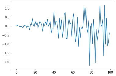
# create a simple white noise with increasing variance
from random import gauss
from random import seed
from matplotlib import pyplot
# seed pseudorandom number generator
seed(1)
# create dataset
data = [gauss(0, i*0.01) for i in range(0,100)]
# plot
pyplot.plot(data)
pyplot.show()
# check correlations of squared observations
from random import gauss
from random import seed
from matplotlib import pyplot
from statsmodels.graphics.tsaplots import plot_acf
# seed pseudorandom number generator
seed(1)
# create dataset
data = [gauss(0, i*0.01) for i in range(0,100)]
# square the dataset
squared_data = [x**2 for x in data]
# create acf plot
# plot_acf(squared_data)
# pyplot.show()
# split into train/test
n_test = 10
train, test = data[:-n_test], data[-n_test:]
# define model
model = arch_model(train, mean='Zero', vol='ARCH', p=15)
# fit model
model_fit = model.fit()
Iteration:      1,   Func. Count:     18,   Neg. LLF: 88229.21081826466
Iteration:      2,   Func. Count:     36,   Neg. LLF: 145.16342486790123
Iteration:      3,   Func. Count:     54,   Neg. LLF: 128.16575632743994
Iteration:      4,   Func. Count:     72,   Neg. LLF: 109.21743453644488
Iteration:      5,   Func. Count:     90,   Neg. LLF: 36.50573961108787
Iteration:      6,   Func. Count:    108,   Neg. LLF: 39.65738666780856
Iteration:      7,   Func. Count:    126,   Neg. LLF: 28.719725578734614
Iteration:      8,   Func. Count:    143,   Neg. LLF: 28.02027082653467
Iteration:      9,   Func. Count:    161,   Neg. LLF: 34.94722141328114
Iteration:     10,   Func. Count:    180,   Neg. LLF: 30.036240932703457
Iteration:     11,   Func. Count:    198,   Neg. LLF: 26.91679507719369
Iteration:     12,   Func. Count:    216,   Neg. LLF: 35.23299109213636
Iteration:     13,   Func. Count:    235,   Neg. LLF: 25.557783947221896
Iteration:     14,   Func. Count:    253,   Neg. LLF: 25.49687793461018
Iteration:     15,   Func. Count:    271,   Neg. LLF: 25.48620371888791
Iteration:     16,   Func. Count:    289,   Neg. LLF: 25.486110427773504
Iteration:     17,   Func. Count:    307,   Neg. LLF: 25.48214947994449
Iteration:     18,   Func. Count:    324,   Neg. LLF: 25.480673701601663
Iteration:     19,   Func. Count:    341,   Neg. LLF: 25.478363191699138
Iteration:     20,   Func. Count:    358,   Neg. LLF: 25.477639119935752
Iteration:     21,   Func. Count:    375,   Neg. LLF: 25.477510674022756
Iteration:     22,   Func. Count:    392,   Neg. LLF: 25.477507680721967
Iteration:     23,   Func. Count:    408,   Neg. LLF: 25.477507647045563
Optimization terminated successfully    (Exit mode 0)
            Current function value: 25.477507680721967
            Iterations: 23
            Function evaluations: 408
            Gradient evaluations: 23
# forecast the test set
yhat = model_fit.forecast(horizon=n_test)
# example of ARCH model
from random import gauss
from random import seed
from matplotlib import pyplot
from arch import arch_model
# seed pseudorandom number generator
seed(1)
# create dataset
data = [gauss(0, i*0.01) for i in range(0,100)]
# split into train/test
n_test = 10
train, test = data[:-n_test], data[-n_test:]
# define model
model = arch_model(train, mean='Zero', vol='ARCH', p=15)
# fit model
model_fit = model.fit()
# forecast the test set
yhat = model_fit.forecast(horizon=n_test)
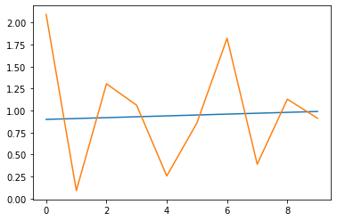
# plot the actual variance
var = [i*0.01 for i in range(0,100)]
pyplot.plot(var[-n_test:])
# plot forecast variance
pyplot.plot(yhat.variance.values[-1, :])
pyplot.show()
Iteration:      1,   Func. Count:     18,   Neg. LLF: 88229.21081826466
Iteration:      2,   Func. Count:     36,   Neg. LLF: 145.16342486790123
Iteration:      3,   Func. Count:     54,   Neg. LLF: 128.16575632743994
Iteration:      4,   Func. Count:     72,   Neg. LLF: 109.21743453644488
Iteration:      5,   Func. Count:     90,   Neg. LLF: 36.50573961108787
Iteration:      6,   Func. Count:    108,   Neg. LLF: 39.65738666780856
Iteration:      7,   Func. Count:    126,   Neg. LLF: 28.719725578734614
Iteration:      8,   Func. Count:    143,   Neg. LLF: 28.02027082653467
Iteration:      9,   Func. Count:    161,   Neg. LLF: 34.94722141328114
Iteration:     10,   Func. Count:    180,   Neg. LLF: 30.036240932703457
Iteration:     11,   Func. Count:    198,   Neg. LLF: 26.91679507719369
Iteration:     12,   Func. Count:    216,   Neg. LLF: 35.23299109213636
Iteration:     13,   Func. Count:    235,   Neg. LLF: 25.557783947221896
Iteration:     14,   Func. Count:    253,   Neg. LLF: 25.49687793461018
Iteration:     15,   Func. Count:    271,   Neg. LLF: 25.48620371888791
Iteration:     16,   Func. Count:    289,   Neg. LLF: 25.486110427773504
Iteration:     17,   Func. Count:    307,   Neg. LLF: 25.48214947994449
Iteration:     18,   Func. Count:    324,   Neg. LLF: 25.480673701601663
Iteration:     19,   Func. Count:    341,   Neg. LLF: 25.478363191699138
Iteration:     20,   Func. Count:    358,   Neg. LLF: 25.477639119935752
Iteration:     21,   Func. Count:    375,   Neg. LLF: 25.477510674022756
Iteration:     22,   Func. Count:    392,   Neg. LLF: 25.477507680721967
Iteration:     23,   Func. Count:    408,   Neg. LLF: 25.477507647045563
Optimization terminated successfully    (Exit mode 0)
            Current function value: 25.477507680721967
            Iterations: 23
            Function evaluations: 408
            Gradient evaluations: 23
# define model
model = arch_model(train, mean='Zero', vol='GARCH', p=15, q=15)
# example of ARCH model
from random import gauss
from random import seed
from matplotlib import pyplot
from arch import arch_model
# seed pseudorandom number generator
seed(1)
# create dataset
data = [gauss(0, i*0.01) for i in range(0,100)]
# split into train/test
n_test = 10
train, test = data[:-n_test], data[-n_test:]
# define model
model = arch_model(train, mean='Zero', vol='GARCH', p=15, q=15)
# fit model
model_fit = model.fit()
# forecast the test set
yhat = model_fit.forecast(horizon=n_test)
# plot the actual variance
var = [i*0.01 for i in range(0,100)]
pyplot.plot(var[-n_test:])
# plot forecast variance
pyplot.plot(yhat.variance.values[-1, :])
pyplot.show()
Iteration:      1,   Func. Count:     33,   Neg. LLF: 134.2317665883839
Iteration:      2,   Func. Count:     70,   Neg. LLF: 95219.42875514245
Iteration:      3,   Func. Count:    103,   Neg. LLF: 544.0651713801462
Iteration:      4,   Func. Count:    136,   Neg. LLF: 359.82260287255474
Iteration:      5,   Func. Count:    169,   Neg. LLF: 120.68468720344026
Iteration:      6,   Func. Count:    202,   Neg. LLF: 57.67993058484209
Iteration:      7,   Func. Count:    235,   Neg. LLF: 37.233844550362896
Iteration:      8,   Func. Count:    268,   Neg. LLF: 44.284908834009805
Iteration:      9,   Func. Count:    301,   Neg. LLF: 30.95579466733611
Iteration:     10,   Func. Count:    334,   Neg. LLF: 26.957522627026123
Iteration:     11,   Func. Count:    366,   Neg. LLF: 31.357987963939777
Iteration:     12,   Func. Count:    400,   Neg. LLF: 30.01446554259058
Iteration:     13,   Func. Count:    433,   Neg. LLF: 28.46108471907541
Iteration:     14,   Func. Count:    466,   Neg. LLF: 27.699881529397864
Iteration:     15,   Func. Count:    499,   Neg. LLF: 26.904390959213814
Iteration:     16,   Func. Count:    532,   Neg. LLF: 25.516070459707
Iteration:     17,   Func. Count:    564,   Neg. LLF: 25.510906607562323
Iteration:     18,   Func. Count:    597,   Neg. LLF: 25.783794390675624
Iteration:     19,   Func. Count:    630,   Neg. LLF: 25.492112073166872
Iteration:     20,   Func. Count:    662,   Neg. LLF: 25.485420508388895
Iteration:     21,   Func. Count:    694,   Neg. LLF: 25.479683744952947
Iteration:     22,   Func. Count:    726,   Neg. LLF: 25.477822001084277
Iteration:     23,   Func. Count:    758,   Neg. LLF: 25.477526070128754
Iteration:     24,   Func. Count:    790,   Neg. LLF: 25.477511628643917
Iteration:     25,   Func. Count:    822,   Neg. LLF: 25.47750785312727
Iteration:     26,   Func. Count:    853,   Neg. LLF: 25.47750781611067
Optimization terminated successfully    (Exit mode 0)
            Current function value: 25.47750785312727
            Iterations: 26
            Function evaluations: 853
            Gradient evaluations: 26

print(model_fit.summary())
                       Zero Mean - GARCH Model Results
==============================================================================
Dep. Variable:                      y   R-squared:                       0.000
Mean Model:                 Zero Mean   Adj. R-squared:                  0.011
Vol Model:                      GARCH   Log-Likelihood:               -25.4775
Distribution:                  Normal   AIC:                           112.955
Method:            Maximum Likelihood   BIC:                           190.449
                                        No. Observations:                   90
Date:                Mon, Feb 15 2021   Df Residuals:                       59
Time:                        18:01:53   Df Model:                           31
                            Volatility Model
========================================================================
                 coef    std err          t      P>|t|  95.0% Conf. Int.
------------------------------------------------------------------------
omega      3.5755e-03      0.163  2.199e-02      0.982 [ -0.315,  0.322]
alpha[1]       0.0000      0.280      0.000      1.000 [ -0.549,  0.549]
alpha[2]   2.8289e-03      0.485  5.836e-03      0.995 [ -0.947,  0.953]
alpha[3]       0.3414      0.413      0.826      0.409 [ -0.469,  1.152]
alpha[4]       0.0000      1.238      0.000      1.000 [ -2.426,  2.426]
alpha[5]       0.0457      0.897  5.101e-02      0.959 [ -1.712,  1.803]
alpha[6]       0.1730      1.134      0.153      0.879 [ -2.050,  2.396]
alpha[7]       0.0000      1.307      0.000      1.000 [ -2.562,  2.562]
alpha[8]       0.1719      0.552      0.311      0.756 [ -0.910,  1.254]
alpha[9]       0.0109      1.844  5.901e-03      0.995 [ -3.603,  3.624]
alpha[10]      0.0000      1.810      0.000      1.000 [ -3.548,  3.548]
alpha[11]      0.0000      0.631      0.000      1.000 [ -1.237,  1.237]
alpha[12]      0.2542      2.076      0.122      0.903 [ -3.815,  4.324]
alpha[13]      0.0000      2.932      0.000      1.000 [ -5.746,  5.746]
alpha[14]      0.0000      1.103      0.000      1.000 [ -2.161,  2.161]
alpha[15]      0.0000      0.773      0.000      1.000 [ -1.514,  1.514]
beta[1]        0.0000      3.707      0.000      1.000 [ -7.266,  7.266]
beta[2]        0.0000      3.724      0.000      1.000 [ -7.300,  7.300]
beta[3]        0.0000      1.360      0.000      1.000 [ -2.665,  2.665]
beta[4]        0.0000      2.043      0.000      1.000 [ -4.004,  4.004]
beta[5]        0.0000      2.186      0.000      1.000 [ -4.285,  4.285]
beta[6]        0.0000      4.237      0.000      1.000 [ -8.305,  8.305]
beta[7]        0.0000      2.941      0.000      1.000 [ -5.765,  5.765]
beta[8]        0.0000      2.371      0.000      1.000 [ -4.647,  4.647]
beta[9]        0.0000      0.921      0.000      1.000 [ -1.806,  1.806]
beta[10]       0.0000      2.166      0.000      1.000 [ -4.245,  4.245]
beta[11]       0.0000      2.381      0.000      1.000 [ -4.668,  4.668]
beta[12]       0.0000      3.735      0.000      1.000 [ -7.321,  7.321]
beta[13]       0.0000      1.904      0.000      1.000 [ -3.732,  3.732]
beta[14]       0.0000      3.439      0.000      1.000 [ -6.739,  6.739]
beta[15]       0.0000      0.499      0.000      1.000 [ -0.978,  0.978]
========================================================================

Covariance estimator: robust
import pandas as pd
df = pd.DataFrame(data)
from tqdm import tqdm
tqdm.pandas()
/Users/ida/opt/anaconda3/lib/python3.8/site-packages/tqdm/std.py:697: FutureWarning: The Panel class is removed from pandas. Accessing it from the top-level namespace will also be removed in the next version
  from pandas import Panel
df['test'] = df.progress_apply(lambda row: 1)
100%|██████████| 1/1 [00:00<00:00, 319.37it/s]