Basic & Econometrics - OLS via Stochastic Gradient Descent

import numpy as np
import pandas as pd
from matplotlib import pyplot as plt
from random import seed, random, gauss
import statsmodels.api as sm

/Users/manguito/.virtualenvs/myEnv/lib/python3.7/site-packages/statsmodels/compat/pandas.py:49: FutureWarning: The Panel class is removed from pandas. Accessing it from the top-level namespace will also be removed in the next version
  data_klasses = (pandas.Series, pandas.DataFrame, pandas.Panel)

OLS with Stochastic Gradient Descent

# Generate data
n = 100
np.random.seed(0)
X = 2.5 * np.random.randn(n) + 1.5   # Array of n values with mean = 1.5, stddev = 2.5
res = 0.5 * np.random.randn(n)       # Generate n residual terms
y = 2 + 0.3 * X + res                  # Actual values of Y

# Create pandas dataframe to store our X and y values
df = pd.DataFrame(
    {'X': X,
     'y': y}
)

# Show the first five rows of our dataframe
df.head()

	X	y
0	5.910131	4.714615
1	2.500393	2.076238
2	3.946845	2.548811
3	7.102233	4.615368
4	6.168895	3.264107

# Calculate the mean of X and y
xmean = np.mean(X)
ymean = np.mean(y)

# Calculate the terms needed for the numator and denominator of beta
df['xycov'] = (df['X'] - xmean) * (df['y'] - ymean)
df['xvar'] = (df['X'] - xmean)**2

# Calculate beta and alpha
beta = df['xycov'].sum() / df['xvar'].sum()
alpha = ymean - (beta * xmean)
print(f'alpha = {alpha}')
print(f'beta = {beta}')

alpha = 2.0031670124623426
beta = 0.3229396867092763

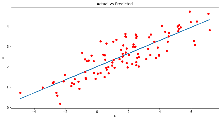
ypred = alpha + beta * X

# Plot regression against actual data
plt.figure(figsize=(12, 6))
plt.plot(X, ypred)     # regression line
plt.plot(X, y, 'ro')   # scatter plot showing actual data
plt.title('Actual vs Predicted')
plt.xlabel('X')
plt.ylabel('y')

plt.show()

# Make a prediction with coefficients
def predict(row, coefficients):
	yhat = coefficients[0]
	for i in range(len(row)-1):
		yhat += coefficients[i + 1] * row[i]
	return yhat
 
# Estimate linear regression coefficients using stochastic gradient descent
def coefficients_sgd(train, l_rate, n_epoch):
	coef = [0.0 for i in range(len(train[0]))]
	for epoch in range(n_epoch):
		sum_error = 0
		for row in train:
			yhat = predict(row, coef)
			error = yhat - row[-1]
			sum_error += error**2
			coef[0] = coef[0] - l_rate * error
			for i in range(len(row)-1):
				coef[i + 1] = coef[i + 1] - l_rate * error * row[i]
		print('>epoch=%d, lrate=%.3f, error=%.3f' % (epoch, l_rate, sum_error))
	return coef
 
# # Calculate coefficients
# dataset = [[1, 1], [2, 3], [4, 3], [3, 2], [5, 5]]
dataset = np.array(df[['X','y']])
l_rate = 0.001
n_epoch = 50
coef = coefficients_sgd(dataset, l_rate, n_epoch)
print(coef)
# df.head()

>epoch=0, lrate=0.001, error=468.733
>epoch=1, lrate=0.001, error=258.425
>epoch=2, lrate=0.001, error=206.738
>epoch=3, lrate=0.001, error=180.854
>epoch=4, lrate=0.001, error=160.966
>epoch=5, lrate=0.001, error=143.946
>epoch=6, lrate=0.001, error=129.113
>epoch=7, lrate=0.001, error=116.156
>epoch=8, lrate=0.001, error=104.837
>epoch=9, lrate=0.001, error=94.950
>epoch=10, lrate=0.001, error=86.314
>epoch=11, lrate=0.001, error=78.772
>epoch=12, lrate=0.001, error=72.184
>epoch=13, lrate=0.001, error=66.430
>epoch=14, lrate=0.001, error=61.404
>epoch=15, lrate=0.001, error=57.015
>epoch=16, lrate=0.001, error=53.181
>epoch=17, lrate=0.001, error=49.832
>epoch=18, lrate=0.001, error=46.907
>epoch=19, lrate=0.001, error=44.352
>epoch=20, lrate=0.001, error=42.120
>epoch=21, lrate=0.001, error=40.171
>epoch=22, lrate=0.001, error=38.468
>epoch=23, lrate=0.001, error=36.980
>epoch=24, lrate=0.001, error=35.681
>epoch=25, lrate=0.001, error=34.545
>epoch=26, lrate=0.001, error=33.554
>epoch=27, lrate=0.001, error=32.687
>epoch=28, lrate=0.001, error=31.930
>epoch=29, lrate=0.001, error=31.269
>epoch=30, lrate=0.001, error=30.691
>epoch=31, lrate=0.001, error=30.186
>epoch=32, lrate=0.001, error=29.745
>epoch=33, lrate=0.001, error=29.359
>epoch=34, lrate=0.001, error=29.022
>epoch=35, lrate=0.001, error=28.728
>epoch=36, lrate=0.001, error=28.471
>epoch=37, lrate=0.001, error=28.246
>epoch=38, lrate=0.001, error=28.049
>epoch=39, lrate=0.001, error=27.877
>epoch=40, lrate=0.001, error=27.727
>epoch=41, lrate=0.001, error=27.596
>epoch=42, lrate=0.001, error=27.481
>epoch=43, lrate=0.001, error=27.381
>epoch=44, lrate=0.001, error=27.293
>epoch=45, lrate=0.001, error=27.216
>epoch=46, lrate=0.001, error=27.149
>epoch=47, lrate=0.001, error=27.090
>epoch=48, lrate=0.001, error=27.039
>epoch=49, lrate=0.001, error=26.994
[1.9381705148304995, 0.335948469233473]

Compare to coefficient estimates from statsmodels

mod = sm.OLS(df.y,sm.add_constant(df['X']))
res = mod.fit()
res.summary()

OLS Regression Results

Dep. Variable:	y	R-squared:	0.715
Model:	OLS	Adj. R-squared:	0.712
Method:	Least Squares	F-statistic:	245.5
Date:	Thu, 10 Dec 2020	Prob (F-statistic):	1.93e-28
Time:	15:28:41	Log-Likelihood:	-75.359
No. Observations:	100	AIC:	154.7
Df Residuals:	98	BIC:	159.9
Df Model:	1
Covariance Type:	nonrobust

	coef	std err	t	P>|t|	[0.025	0.975]
const	2.0032	0.062	32.273	0.000	1.880	2.126
X	0.3229	0.021	15.669	0.000	0.282	0.364

Omnibus:	5.184	Durbin-Watson:	1.995
Prob(Omnibus):	0.075	Jarque-Bera (JB):	3.000
Skew:	0.210	Prob(JB):	0.223
Kurtosis:	2.262	Cond. No.	3.73

Warnings:
[1] Standard Errors assume that the covariance matrix of the errors is correctly specified.