Machine Learning - Regularized regression

import numpy as np
import matplotlib.pyplot as plt
from sklearn import linear_model

# X is the 10x10 Hilbert matrix
X = 1. / (np.arange(1, 11) + np.arange(0, 10)[:, np.newaxis])
y = np.ones(10)

# #############################################################################
# Compute paths

n_alphas = 200
alphas = np.logspace(-10, -2, n_alphas)

coefs = []
for a in alphas:
    ridge = linear_model.Ridge(alpha=a, fit_intercept=False)
    ridge.fit(X, y)
    coefs.append(ridge.coef_)

# #############################################################################
# Display results

ax = plt.gca()

ax.plot(alphas, coefs)
ax.set_xscale('log')
ax.set_xlim(ax.get_xlim()[::-1])  # reverse axis
plt.xlabel('alpha')
plt.ylabel('weights')
plt.title('Ridge coefficients as a function of the regularization')
plt.axis('tight')
plt.show()

# Author: Fabian Pedregosa <fabian.pedregosa@inria.fr>
#         Alexandre Gramfort <alexandre.gramfort@inria.fr>
# License: BSD 3 clause

import numpy as np
import matplotlib.pyplot as plt

from sklearn import linear_model
from sklearn import datasets

X, y = datasets.load_diabetes(return_X_y=True)

print("Computing regularization path using the LARS ...")
_, _, coefs = linear_model.lars_path(X, y, method='lasso', verbose=True)

xx = np.sum(np.abs(coefs.T), axis=1)
xx /= xx[-1]

plt.plot(xx, coefs.T)
ymin, ymax = plt.ylim()
plt.vlines(xx, ymin, ymax, linestyle='dashed')
plt.xlabel('|coef| / max|coef|')
plt.ylabel('Coefficients')
plt.title('LASSO Path')
plt.axis('tight')
plt.show()

Computing regularization path using the LARS ...
.

# Author: Alexandre Gramfort <alexandre.gramfort@inria.fr>
# License: BSD 3 clause

from itertools import cycle
import numpy as np
import matplotlib.pyplot as plt

from sklearn.linear_model import lasso_path, enet_path
from sklearn import datasets


X, y = datasets.load_diabetes(return_X_y=True)


X /= X.std(axis=0)  # Standardize data (easier to set the l1_ratio parameter)

# Compute paths

eps = 5e-3  # the smaller it is the longer is the path

print("Computing regularization path using the lasso...")
alphas_lasso, coefs_lasso, _ = lasso_path(X, y, eps=eps, fit_intercept=False)

print("Computing regularization path using the positive lasso...")
alphas_positive_lasso, coefs_positive_lasso, _ = lasso_path(
    X, y, eps=eps, positive=True, fit_intercept=False)
print("Computing regularization path using the elastic net...")
alphas_enet, coefs_enet, _ = enet_path(
    X, y, eps=eps, l1_ratio=0.8, fit_intercept=False)

print("Computing regularization path using the positive elastic net...")
alphas_positive_enet, coefs_positive_enet, _ = enet_path(
    X, y, eps=eps, l1_ratio=0.8, positive=True, fit_intercept=False)

# Display results

plt.figure(1)
colors = cycle(['b', 'r', 'g', 'c', 'k'])
neg_log_alphas_lasso = -np.log10(alphas_lasso)
neg_log_alphas_enet = -np.log10(alphas_enet)
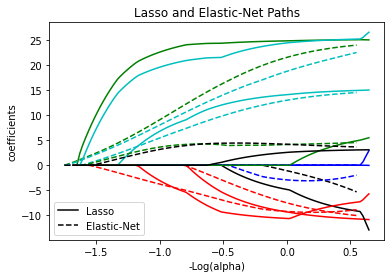
for coef_l, coef_e, c in zip(coefs_lasso, coefs_enet, colors):
    l1 = plt.plot(neg_log_alphas_lasso, coef_l, c=c)
    l2 = plt.plot(neg_log_alphas_enet, coef_e, linestyle='--', c=c)

plt.xlabel('-Log(alpha)')
plt.ylabel('coefficients')
plt.title('Lasso and Elastic-Net Paths')
plt.legend((l1[-1], l2[-1]), ('Lasso', 'Elastic-Net'), loc='lower left')
plt.axis('tight')


plt.figure(2)
neg_log_alphas_positive_lasso = -np.log10(alphas_positive_lasso)
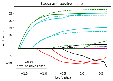
for coef_l, coef_pl, c in zip(coefs_lasso, coefs_positive_lasso, colors):
    l1 = plt.plot(neg_log_alphas_lasso, coef_l, c=c)
    l2 = plt.plot(neg_log_alphas_positive_lasso, coef_pl, linestyle='--', c=c)

plt.xlabel('-Log(alpha)')
plt.ylabel('coefficients')
plt.title('Lasso and positive Lasso')
plt.legend((l1[-1], l2[-1]), ('Lasso', 'positive Lasso'), loc='lower left')
plt.axis('tight')


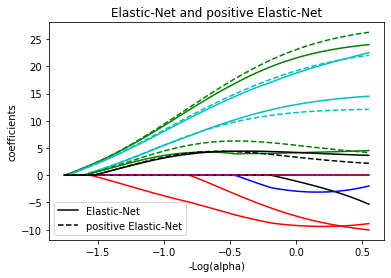
plt.figure(3)
neg_log_alphas_positive_enet = -np.log10(alphas_positive_enet)
for (coef_e, coef_pe, c) in zip(coefs_enet, coefs_positive_enet, colors):
    l1 = plt.plot(neg_log_alphas_enet, coef_e, c=c)
    l2 = plt.plot(neg_log_alphas_positive_enet, coef_pe, linestyle='--', c=c)

plt.xlabel('-Log(alpha)')
plt.ylabel('coefficients')
plt.title('Elastic-Net and positive Elastic-Net')
plt.legend((l1[-1], l2[-1]), ('Elastic-Net', 'positive Elastic-Net'),
           loc='lower left')
plt.axis('tight')
plt.show()

Computing regularization path using the lasso...
Computing regularization path using the positive lasso...
Computing regularization path using the elastic net...
Computing regularization path using the positive elastic net...